End To End Machine Learning Project To Predict Housing Prices In California

28 min readMay 26, 2021

Having a keen interest in data science and real estate I thought it would be a great idea to combine my two interests into an interesting machine learning project in which I was aiming to develop and deploy an application to predict the prices of houses in California. Why California housing prices you may ask? Simply, because there is a very rich and publicly available dataset from the 1990 California census which we can easily access for model training. Yes, of course, this may not help us with predicting current housing prices, however it does provide an accessible introductory dataset for teaching people about the basics of machine learning.

Furthermore, the dataset isn’t entirely clean! Thus, there are some preprocessing steps required which you will see as we begin to explore the dataset. This is a great practice!

In this article I will be focusing solely on the process from data exploration to building an end to end machine learning pipeline. We will look at the problem in depth and from several angles. We will also consider many different approaches to tackling the problem given certain scenarios. My goal is to not just provide a solution to this particular machine learning problem, but to incorporate many other ideas so that I can provide you with a framework which you take and apply to many other machine learning problems. Therefor, I would encourage you to keep an open mind as you read the article and try to think of ways that you could apply these solutions to your own projects.

All of the key steps required in the process of model development are outlined below in the table of contents.

Download the data
Exploratory Data Analysis
Data Cleaning
Data Preprocessing
Select and train a machine learning model
Fine tune the model
Build a pipeline

P.S: In the near future I am planning on writing a second article where I will be focusing on how to put this machine learning solution in an application and deploy it on Heroku.

The application is deployed and available here: https://houses-bts.herokuapp.com/

All of the code and data for this project can be seen on my Github Repository for this project here: https://github.com/lukeclarke12/california_housing_project

Now, with all that said lets get to it!

1. Download the Data

Before we do anything let’s first import all of the libraries and make any necessary adjustments that will be required for this project.

In typical environments your data would be available in a relational database (or some other common datastore) and spread across multiple tables/documents/files. To access it, you would first need to get your credentials and access authorizations, and familiarize yourself with the data schema.

In this project, however, things are much simpler: you will just download a single compressed file, housing.tgz, (available on my github) which contains a comma-separated value (CSV) file called housing.csv with all the data.

You could use your web browser to download it, and run tar xzf housing.tgz to decompress the file and extract the CSV file, but it is preferable to create a small function to do that. It is useful in particular if data changes regularly, as it allows you to write a small script that you can run whenever you need to fetch the latest data (or you can set up a scheduled job to do that automatically at regular intervals). Automating the process of fetching the data is also useful if you need to install the dataset on multiple machines.

Now we can create a function to load the CSV into Pandas and make it return a Pandas DataFrame of our housing dataset.

And, that is step one, getting the data, complete! Lets keep going.

2. Exploratory Data Analysis

Firstly, lets use the .info() method to retrieve some information about the dataset. Here we can get a quick snapshot of the current state of the dataset. How many columns and rows to we have? What do the column variables refer to? What data types do we have? Are they numerical or categorical? Do we have any null values?

Here we have nine features and one target variable which is the median_house_value.

1. longitude: A measure of how far west a house is; a higher value is farther west.

2. latitude: A measure of how far north a house is; a higher value is farther north

3. housing_median_age: Median age of a house within a block; a lower number is a newer building

4. total_rooms: Total number of rooms within a block

5. total_bedrooms: Total number of bedrooms within a block

6. population: Total number of people residing within a block

7. households: Total number of households, a group of people residing within a home unit, for a block

8. median_income: Median income for households within a block of houses (measured in tens of thousands of US Dollars)

9. median_house_value: Median house value for households within a block (measured in US Dollars). This is the target variable.

10. ocean_proximity: Location of the house w.r.t ocean/sea

Initially, I can immediately see that there are null values present in the total_bedrooms column. This is something that we will handle shortly, but it is good have this in mind from the start.

Furthermore, It seems that all data columns are numerical, but there is one which is an object. It should surely be some sort of text, perhaps a category. Try to check which categories those are and how many districts belong to that category by using the value_counts() method.

Next, lets print a statistical summary of the dataset. It is important for us to get a good understanding of the characteristics of our data. We want to know more specifically what are the min, max, mean, standard deviation, upper and lower bounds and count of all the variables within our dataset. This information is important firstly for determining the general characteristics of our data, secondly, for determining the outliers we have in our data and it will give also us a better idea as to how we need to prepare our data for training later on.

Another thing we need to understand right from the start are the distributions underlying our dataset. When training a machine learning model for optimisation ideally we want all of our variables to be as close as possible to a normal distribution. If this is not the case then maybe we can perform some transforms on the data in order to transform it into having a normal distribution.

Looking at these plots what do you think are the questions you need to be asking yourself?

Here are some of the questions I am pondering….

Is the median income expressed in dollars?
And the median age and house value? How are they expressed?
Do all the attributes have the same scale?
Most of histograms are skewed… how would this affect learning?

Well to answer these questions…..

First, the median income attribute does not look like it is expressed in US dollars (USD). Let’s imagine that after checking with your team that collected the data, you are told that the data has been scaled and capped at 15 (actually 15.0001) for higher median incomes, and at 0.5 (actually 0.4999) for lower median incomes. Working with preprocessed attributes is common in Machine Learning, and it is not necessarily a problem, but you should try to understand how the data was computed.
The housing median age and the median house value were also capped. The latter may be a serious problem since it is your target attribute (your labels). Your Machine Learning algorithms may learn that prices never go beyond that limit. You need to check with your client team (the team that will use your system’s output) to see if this is a problem or not. If they tell you that they need precise predictions even beyond 500,000 dollars, then you have mainly two options:

Collect proper labels for the districts whose labels were capped.
Remove those districts from the training set (and also from the test set, since your system should not be evaluated poorly if it predicts values beyond $500,000).

3. These attributes have very different scales and this is a problem.

4. Finally, many histograms are tail heavy: they extend much farther to the right of the median than to the left. This may make it a bit harder for some Machine Learning algorithms to detect patterns. We will try transforming these attributes later on to have more bell-shaped distributions.

We will discuss how to deal with these issues later in the article for now we are just exploring the data and getting an idea of the big picture and the steps that we will need to take later in order to tackle this problem. This exploratory data analysis step is all about gathering information and understanding the data!

Before going any further lets create a test set

It may sound strange to voluntarily set aside part of the data at this stage. After all, you have only taken a quick glance at the data, and surely you should learn a whole lot more about it before you decide what algorithms to use, right?

This is true, but your brain is an amazing pattern detection system, which means that it is highly prone to overfitting: if you look at the test set, you may stumble upon some seemingly interesting pattern in the test data that leads you to select a particular kind of Machine Learning model.

When you estimate the generalisation error using the test set, your estimate will be too optimistic and you will launch a system that will not perform as well as expected. This is called data snooping bias.

Creating a test set is theoretically quite simple: just pick some instances randomly, typically 20% of the dataset, and set them aside. This can easily be done using Sklearns built in train_test_split() function.

Lets talk about sampling

So far we have considered purely random sampling methods. This is generally fine if your dataset is large enough (especially relative to the number of attributes), but if it is not, you run the risk of introducing a significant sampling bias.

When a survey company decides to call 1,000 people to ask them a few questions, they don’t just pick 1,000 people randomly in a phone booth. They try to ensure that these 1,000 people are representative of the whole population. For example, the US population is composed of 51.3% female and 48.7% male, so a well-conducted survey in the US would try to maintain this ratio in the sample: 513 female and 487 male.

This is called STRATIFIED SAMPLING: the population is divided into homogeneous subgroups called strata, and the right number of instances is sampled from each stratum to guarantee that the test set is representative of the overall population.

Suppose you chatted with experts who told you that the median income is a very important attribute to predict median housing prices. It is a variable that defines population composition in this dataset as well as female/male does for the US population. You may want to ensure that the test set is representative of the various categories of incomes in the whole dataset. Since the median income is a continuous numerical attribute, you first need to create an income category attribute.

Most median income values are clustered around 2–5 (tens of thousands of dollars), but some median incomes go far beyond 6. It is important to have a sufficient number of instances in your dataset for each stratum, or else the estimate of the stratum’s importance may be biased.

This means that you should not have too many strata, and each stratum should be large enough. The following code uses the pd.cut() function to create an income category attribute with five categories of median income (labels 1 to 5).

Now we are ready to do stratified sampling based on the income category that we have just created using StratifiedShuffleSplit class.

Let’s check the proportions of the income category proportions in the overall dataset, in the test set generated with stratified sampling, and in a test set generated using purely random sampling.

As you can see, the test set generated using stratified sampling has income category proportions almost identical to those in the full dataset, whereas the test set generated using purely random sampling is quite skewed.

Now let’s drop the income_cat attribute from the stratified sets, since we only needed it for actually stratifying the dataset.

Visualising The Data

First, make sure you have put the test set aside and you are only exploring the training set. Also, if the training set is very large, you may want to sample an exploration set, to make manipulations easy and fast.

In our case, the set is quite small so you can just work directly on the full set. Let’s create a copy so you can play with it without harming the training set.

Next we will plot a simple plot of the dataset using its longitude and latitude. However, we want to try to do it in a way that will reveal some information and patterns (population, house prices) in the same plot.

This is an example of a bad visualisation of our data as it is not revealing a lot of useful information to us.

This is a slightly better visualisation as it gives us an idea as to where the more expensive houses are located. You can quickly get the impression that the more expensive houses are located close to the Ocean, and in the cities San Diego, Los Angelas and San Francisco.

This is an example of a great visualisation plot!

If you plot it correctly, you will see that there are different patterns and areas of different price density. You will see that houses are more expensive as they get closer and closer to ocean and where there is a lot of population.

It will probably be useful to use a clustering algorithm to detect the main clusters, and add new features that measure the proximity to the cluster centers. The ocean proximity attribute may be useful as well, although in Northern California the housing prices in coastal districts are not too high, so it is not a simple rule.

Looking For Correlations

It is important to analyse the correlation coefficients between variables. When building machine learning models we are aiming to look for features that have a significant correlation ( be it positive or negative ) with our target variable in this case the median house value. Provided that the “correlation implies causation” these features will be important in determining the target variable and in increasing the accuracy of our model.

However, we also want to avoid introducing multi-collinearity into our model. This is when we have a significant correlation between the features within our model. If we have multi-collinearity in our model it will negatively affect the balance of our model coefficients leading to a more inaccurate model.

Since the dataset is not too large, you can easily compute the standard correlation coefficient (also called Pearson’s r) between every pair of attributes using the corr() method:

You can see how each variable correlates with “median_house_value” which is what is interesting for us:

The correlation coefficient ranges from –1 to 1.

When it is close to 1, it means that there is a strong positive correlation; for example, the median house value tends to go up when the median income goes up. When the coefficient is close to –1, it means that there is a strong negative correlation; you can see a small negative correlation between the latitude and the median house value (i.e., prices have a slight tendency to go down when you go north). Finally, coefficients close to zero mean that there is no linear correlation.

Below there is an image with the standard correlation coefficient (Pearson’s r) of various datasets:

We can also use plot a scatter matrix to plot graphs for each of the following attributes:

median_house_value
median_income
total_rooms
housing_median_age

Note: The correlation coefficient only measures linear correlations (if x goes up, then y generally goes up/down). It may completely miss out on nonlinear relationships (e.g., if x is close to zero then y generally goes up).

Note how all the plots of the bottom row have a correlation coefficient equal to zero despite the fact that their axes are clearly not independent: these are examples of nonlinear relationships.

Exploring Different Attribute Combinations

Hopefully the previous sections gave you an idea of a few ways you can explore the data and gain insights. You identified a few data quirks that you may want to clean up before feeding the data to a Machine Learning algorithm, and you found interesting correlations between attributes, in particular with the target attribute.

You also noticed that some attributes have a tail-heavy distribution, so you may want to transform them (e.g., by computing their logarithm). Of course, your mileage will vary considerably with each project but the general ideas are similar.

One last thing you may want to do before actually preparing the data for Machine Learning algorithms is to try out various attribute combinations. For example, the total number of rooms in a district is not very useful if you don’t know how many households there are.

What you really want is the number of rooms per household. Similarly, the total number of bedrooms by itself is not very useful: you probably want to compare it to the number of rooms. And the population per household also seems like an interesting attribute combination to look at. Let’s create these new attributes:

Now lets recreate the correlation matrix with the new values.

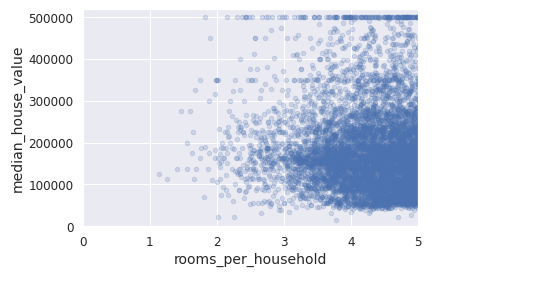
Apparently houses with a lower bedroom/room ratio tend to be more expensive. The number of rooms per household is also more informative than the total number of rooms in a district — obviously the larger the houses, the more expensive they are.

This round of exploration does not have to be absolutely thorough; the POINT is to start off on the right foot and quickly gain insights that will help you get a first reasonably good model prototype.

But this is an iterative process: once you get a model prototype up and running, you can analyse its output to gain more insights and come back to this exploration step!

If you have followed me this far you are doing great! This brings us to the end of our initial exploratory data analysis step. Now it is time to start cleaning and preparing the data for our machine learning algorithm!

Preparing the Data for Machine Learning Algorithms

It’s time to prepare the data for your Machine Learning algorithms. Instead of just doing this manually, you should write functions to do that, for several good reasons:

This will allow you to reproduce these transformations easily on any dataset (e.g., the next time you get a fresh dataset).
You will gradually build a library of transformation functions that you can reuse in future projects.
You can use these functions in your live system to transform the new data before feeding it to your algorithms.
This will make it possible for you to easily try various transformations and see which combination of transformations works best.

3. Data Cleaning

First let’s revert to a clean training set (by copying strat_train_set once again), and let’s separate the predictors and the labels since we don’t necessarily want to apply the same transformations to the predictors and the target values (note that drop() creates a copy of the data and does not affect strat_train_set):

Dealing with Null Values

We noticed earlier that we had missing values (NaN) in our dataset in the total_bedrooms column:

Most Machine Learning algorithms cannot work with missing features, so let’s create a few functions to take care of them. You might have noticed that the total_bedrooms attribute has some missing values, so let’s fix this. You have three options:

Get rid of the corresponding districts.
Get rid of the whole attribute.
Set the values to some value (zero, the mean, the median, etc.)

Beware that if you use fillna() you should compute the median value on the training set, and use it to fill the missing values in the training set, but also don’t forget to save the median value that you have computed. You will need it later to replace missing values in the test set when you want to evaluate your system, and also once the system goes live to replace missing values in new data.

Option 1:

Option 2:

Option 3:

More often then not, replacing Nan values with the median is the best course of action. Especially when we have a smaller dataset and we don’t want to lose any of our precious data. If we have a very large dataset it is fine to just drop the Nan values provided there is only a small number of them. It is better to replace the Nan values with the median rather then the mean as the median is less affected when the distribution of our dataset is skewed.

If the data is skewed to the left as in the graph below the mean will also skew to the left.

If the data is skewed to the right the mean will also skew to the right.

If the data is perfectly normally distributed Mean = Median = Mode, and it doesn’t matter if we replace with the mean or the median.

However, unfortunately this is not always the case!

Dealing with Outliers

We don’t have outliers in this dataset as I already outlined that the data has been scaled and capped at 15 for higher median incomes, and at 0.5 for lower median incomes. However, I think it is important to discuss how to deal with outliers if they are present in your data as this is a very common issue. Outliers are something you always need to check for in your data when approaching a machine learning problem and handle them appropriately if they are present. Machine learning algorithms are sensitive to the range and distribution of attribute values. Data outliers can spoil and mislead the training process resulting in longer training times, less accurate models and ultimately poorer results.

We can handle outliers in the exact same way as we handle null values. Again, with outliers it is even more important to use the median as a replacement value over the mean as outliers affect the mean of our data. When we replace the outliers with a new value the mean of our data will also change, however the median is unaffected.

There is also one more way to deal with outliers that called capping! Which is what has previously been done to our housing data in this case. This is the optimal method of dealing with outliers. Here we first identify the upper and lower bounds of our data. This is generally done by calculating 1.5*IQR (Inter-quartile range) above and below the mean. All data points that fall outside our upper and lower bounds are considered outliers and need to be replaced by the upper or lower bound.

Data points that fall above the upper bound are replaced with the upper bound value (1.5*IQR) and every data point that falls below the lower bound are replaced with the lower bound value (-1.5*IQR).

Imputer

Sklearn provides a handy class to take care of missing values: Imputer. Here is how to use it. First, you need to create an Imputer instance, specifying that you want to replace each attribute’s missing values (or outlier) with the median of that attribute.

However, the median can only be computed on numerical attributes, we need to create a copy of the data without the text attribute ocean_proximity.

Remove the text attribute because median can only be calculated on numerical attributes:

The Imputer has simply computed the median of each attribute and stored the result in its statistics_ instance variable. Only the total_bedrooms attribute had missing values, but we cannot be sure that there won’t be any missing values in new data after the system goes live, so it is safer to apply the imputer to all the numerical attributes.

Now you can use this “trained” imputer to transform the training set by replacing missing values by the learned medians.

The result is a plain Numpy array containing the transformed features. If you want to put it back into a Pandas DataFrame, it’s simple.

4. Data Preprocessing

Handling Text and Categorical Variables

But wait a second, what about our ocean_proximity variable? We need to convert it to labels and put it back to the DataFrame. We can do this using OneHotEncoders, OrdinalEncoders… you name it.

Now let’s preprocess the categorical input feature, ocean_proximity:

Let’s use OneHotEncoder from sklearn.preprocessing and fit_transform the variable. and then print some of the entries. OneHotEncoder is a way of encoding text variables with numbers so that a machine can understand the text variable.

For example, there are five possible options in our dataset for the Ocean Proximity variable:

The OneHotEncoder class will return an array in the place of each row. In this case if the category in a row was <1H Ocean the array returned would be [1, 0, 0, 0, 0]. If it was Near Ocean the array would be [0, 0, 1, 0, 0].

The 1 signals to the machine which category is present in the row instance.

By default, the OneHotEncoder class returns a sparse array, but we can convert it to a dense array if needed by calling the toarray() method.

You can access the categories from OneHotEncoder as such:

Custom Transformers

Transformers are part of Sklearn’s API, the transformation is performed by the transform() method with the dataset to transform as a parameter. It returns the transformed dataset. This transformation generally relies on the learned parameters, as is the case for an imputer. All transformers also have a convenience method called fit_transform(), which directly fits and transforms the data.

Although Sklearn provides many useful transformers, you will need to write your own for tasks such as custom cleanup operations or combining specific attributes. You will want your transformer to work seamlessly with Sklearn functionalities (such as pipelines), and since Sklearn relies on duck typing (not inheritance), all you need is to create a class and implement three methods: fit() (returning self), transform(), and fit_transform().

You can get the last one for free by simply adding TransformerMixin as a base class. Also, if you add BaseEstimator as a base class (and avoid args and *kargs in your constructor) you will get two extra methods (get_params() and set_params()) that will be useful for automatic hyper-parameter tuning. For example, here is a small transformer class that adds the combined attributes we discussed earlier:

In this example the transformer has one hyper-parameter, add_bedrooms_per_room, set to True by default (it is often helpful to provide sensible defaults).

This hyper-parameter will allow you to easily find out whether adding this attribute helps the Machine Learning algorithms or not. More generally, you can add a hyper-parameter to gate any data preparation step that you are not 100% sure about.

The more you automate these data preparation steps, the more combinations you can automatically try out, making it much more likely that you will find a great combination (and saving you a lot of time).

Feature Scaling

One of the most important transformations you need to apply to your data is feature scaling. With few exceptions, Machine Learning algorithms don’t perform well when the input numerical attributes have very different scales. This is the case for the housing data: the total number of rooms ranges from about 6 to 39,320, while the median incomes only range from 0 to 15. Note that scaling the target values is generally not required.

There are two common ways to get all attributes to have the same scale: min-max scaling and standardization.

Min-max scaling (many people call this normalization) is quite simple: values are shifted and rescaled so that they end up ranging from 0 to 1.

Standardization is quite different: first it subtracts the mean value (so standardized values always have a zero mean), and then it divides by the variance so that the resulting distribution has unit variance. We can easily scale our data using the built in StandardScaler() class from sklearn.

Now lets build a full preprocessing pipeline that will:

Impute null values with the median
Create the combined attributes using the CombinedAttributesAdder() class we wrote
Scale our data using the StandardScaler() class
Apply fit transform to it
OneHotEncode the Ocean Proximity variable

To do this we will use the pipeline class from Sklearn that will execute each one of these tasks in a sequential manner. We will create two separate pipelines to handle our numerical and categorical variables independently, and we will then create a “full pipeline” with these two pipelines embedded into it.

Now our data is finally ready to be ingested by a machine learning model. It is time for the exciting part. Let’s continue!

5. Select and Train a Machine Learning Model

At last! You framed the problem, you got the data and explored it, you sampled a training set and a test set, and you wrote transformation pipelines to clean up and prepare your data for Machine Learning algorithms automatically. You are now ready to select and train a Machine Learning model.

The Bias Variance Tradeoff

Fundamentally, the question of “the best model” is about finding a sweet spot in the tradeoff between bias and variance. Consider the following figure, which presents two regression fits to the same dataset:

It is clear that neither of these models is a particularly good fit to the data, but they fail in different ways.

The model on the left attempts to find a straight-line fit through the data. Because the data are intrinsically more complicated than a straight line, the straight-line model will never be able to describe this dataset well. Such a model is said to underfit the data: that is, it does not have enough model flexibility to suitably account for all the features in the data; another way of saying this is that the model has high bias.

The model on the right attempts to fit a high-order polynomial through the data. Here the model fit has enough flexibility to nearly perfectly account for the fine features in the data, but even though it very accurately describes the training data, its precise form seems to be more reflective of the particular noise properties of the data rather than the intrinsic properties of whatever process generated that data. Such a model is said to overfit the data: that is, it has so much model flexibility that the model ends up accounting for random errors as well as the underlying data distribution; another way of saying this is that the model has high variance.

When trying to decide on an ML model you want to develop a simple baseline model. If this model performs sufficiently well then we don’t need to use a more complex model. However, if the model underfits the data then we can move towards more complex models remaining cautious as we don’t want our model to overfit the data. Again, we are looking for the sweet spot!

Training and Evaluating on the Training Set

Thanks to all our hard work, now it is extremely simple to deal with this dataset. Lets start off with a simple linear regression model.

Now let’s try few instances from the training set to do some inferences. We just skip through all the crazy data wrangling and just apply the pipeline we created.

Compare against the actual values:

It works more or less but we could certify it by analysing the mean squared error and the mean absolute error.

Lets create some util functions to display scores more easily:

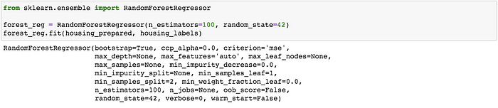
Now lets try a more complex model. A random forest regressor perhaps.

Cross Validation

One disadvantage of using a holdout set for model validation is that we have lost a portion of our data to the model training. In the above case, half the dataset does not contribute to the training of the model! This is not optimal, and can cause problems — especially if the initial set of training data is small.

One way to address this is to use cross-validation; that is, to do a sequence of fits where each subset of the data is used both as a training set and as a validation set. Visually, it might look something like this:

Here we split the data into five groups, and use each of them in turn to evaluate the model fit on the other 4/5 of the data. This would be rather tedious to do by hand, and so we can use Sklearn’s cross_val_score convenience routine to do it succinctly.

In our case lets run a cross validation with 10 folds!

Keeping Your Experiments Saved

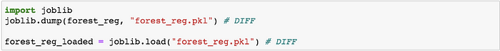
You should save every model you experiment with, so you can come back easily to any model you want. Make sure you save both the hyper parameters and the trained parameters, as well as the cross-validation scores and perhaps the actual predictions as well. This will allow you to easily compare scores across model types, and compare the types of errors they make. You can easily save Sklearn models by using Python’s pickle module, or using sklearn.externals.joblib, which is more efficient at serializing large NumPy arrays.

6. Fine Tuning The Model

GridSearchCV

GridSearchCV is a library function that is a member of Sklearn’s model_selection package. It helps to loop through predefined hyper parameters and fit your estimator (model) on your training set. So, in the end, you can automatically select the best parameters from the listed hyper parameters.

The best hyper-parameter combination found:

Let’s look at the score of each hyper-parameter combination tested during the grid search:

Introducing RandomizedSearchCV

The grid search approach is fine when you are exploring relatively few combinations, like in the previous example, but when the hyper-parameter search space is large, it is often preferable to use RandomizedSearchCV instead.

This class can be used in much the same way as the GridSearchCV class, but instead of trying out all possible combinations, it evaluates a given number of random combinations by selecting a random value for each hyper-parameter at every iteration. This approach has two main benefits:

If you let the randomised search run for, say, 1,000 iterations, this approach will explore 1,000 different values for each hyper-parameter (instead of just a few values per hyper-parameter with the grid search approach).
You have more control over the computing budget you want to allocate to hyper‐ parameter search, simply by setting the number of iterations.

Analyse the Best Models and their errors

You will often gain good insights on the problem by inspecting the best models. For example, the RandomForestRegressor can indicate the relative importance of each attribute for making accurate predictions

With this information, you may want to try dropping some of the less useful features (e.g., apparently only one ocean_proximity category is really useful, so you could try dropping the others).

You should also look at the specific errors that your system makes, then try to understand why it makes them and what could fix the problem (adding extra features or, on the contrary, getting rid of uninformative ones, cleaning up outliers, etc.).

Evaluate your final system on the test set

Evaluate the final system on the test set. There is nothing special about this process; just get the predictors and the labels from your test set, run your full_pipeline to transform the data (call transform(), not fit_transform()!), and evaluate the final model on the test set. Print the performance metrics that you have chosen.

7. Building a Pipeline

A full pipeline with both preparation and prediction and model persistence

Now, let’s wrap it all up and create a pipeline that prepares data and applies your algorithm. Then run and fit and predict some data through it. Alternatively, save model with joblib for next time.

Well if you made it this far congratulations. Give yourself a pat on the back! It was a long road. I hope you learned something. We started at the beginning downloading the data and knowing very little about it, to conducting an in depth data exploration, discovering and dealing with all the underlying problems within the dataset, exploring different machine learning models as a solution and incorporating the whole process into and end to end prediction pipeline. If you enjoyed the article please give it a thumbs up. If you have any questions please leave and comment.

Have a good day!